mND: Gene relevance based on multiple evidences in complex networks.
2024-04-09
mND.Rmd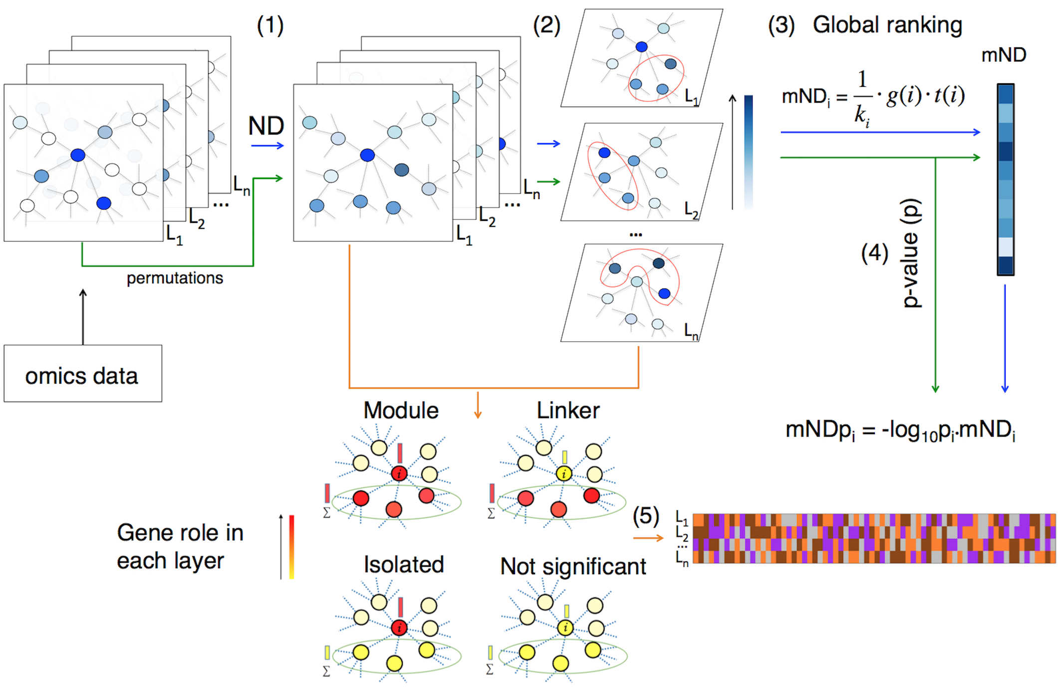
Introduction
This document describes the R package mND (Di Nanni et al. 2019), a new network diffusion based method for integrative multi-omics analysis.
Installation
The package can be installed from within R:
install.packages(c("devtools", "igraph"))
devtools::install_github("emosca-cnr/mND", build_vignettes = TRUE)
library(mND)
Definition of the input matrices
The analysis requires the following inputs:
- \(\mathbf{W}\), an \(N \times N\) normalized adjacency matrix, which represents the interactions between genes, e.g.:
## 5 x 5 sparse Matrix of class "dgCMatrix"
##              A1BG        A2M A4GALT A4GNT AAAS
## A1BG   .          0.01022807      .     .    .
## A2M    0.01022807 .               .     .    .
## A4GALT .          .               .     .    .
## A4GNT  .          .               .     .    .
## AAAS . . . . .- \(\mathbf{X}_0\), a \(N \times m\) matrix with column vectors that contain gene-related quantities, e.g.:
##                L1         L2
## A1BG   0.00000000 0.00000000
## A2M    0.02857143 8.96179484
## A4GALT 0.00000000 1.55085417
## A4GNT  0.00000000 0.00000000
## AAAS   0.00000000 0.05228165
## AACS   0.00000000 1.22029740
## AADAT  0.00000000 1.90713768
## AAK1   0.00000000 0.15747190
## AAMP   0.00000000 0.56363846
## AANAT 0.00000000 0.00000000IMPORTANT:
- the two matrices must be defined over the same identifiers;
- the normalization of the adjacency matrix must be done by means of
the function
NPATools::normalize_adj_mat(), which requires a symmetric binary adjacency matrix; - the relevance of the genes corresponding to the rows of \(\mathbf{X}_0\) is proportional to the values, that is, the higher the better; negative values are not allowed.
Case study: integration of mutation and expression changes in breast cancer
As proof of principle, mND is applied to find functionally related genes on the basis of gene mutations (\(L_1\)) and gene expression variation (\(L_2\)) in breast cancer (BC).
Somatic mutations and gene expression data from matched tumour-normal samples (blood for SM and solid tissue for GE) were collected from The Cancer Genome Atlas (TCGA) (Tomczak et al. 2015) for BC, using the R package TCGAbiolinks (Colaprico et al. 2015) and considering the human genome version 38 (hg38).
Mutation Annotation Format files were obtained from 4 pipelines: Muse (Fan et al. 2016), Mutect2 (Cibulskis et al. 2013), SomaticSniper (Larson et al. 2011), Varscan2 (Koboldt et al. 2012). Only mutation sites detected by at least two variant callers were considered. Gene mutation frequencies (\(f\)) were calculated as the fraction of subjects in which a gene was associated with at least one mutation.
Gene expression data were obtained using the TCGA workflow ``HTSeq-Counts’’. The R package limma (Ritchie et al. 2015) was used to normalize and quantify differential expression in matched tumor-normal samples, yielding log-fold changes, the corresponding p-values and FDRs (BH method).
We obtained the normalized adjacency matrix (\(W\)) using the interactions available in STRING (Szklarczyk et al. 2015), while \(X0\) matrix was defined as the two column vectors: \(x_1 = f\) and \(x_2 = -log_{10}(FDR)\).
Permutations
A set of \(k\) permutations can be
created using the two functions of NPATools perm_vertices()
and perm_X0():
vert_deg <- setNames(rowSums(sign(W)), rownames(W))
perms <- perm_vertices(vert_deg, method = "d", k = 99, cut_par = 9, bin_type = "number")
X0_perm <- perm_X0(X0, perms = perms)
Here’s how X0_perm should look like:
## [[1]]
##                L1         L2
## A1BG   0.00000000 0.00000000
## A2M    0.02857143 8.96179484
## A4GALT 0.00000000 1.55085417
## A4GNT  0.00000000 0.00000000
## AAAS   0.00000000 0.05228165
## AACS   0.00000000 1.22029740
##
## [[2]]
##        L1         L2
## A1BG    0  0.8572643
## A2M     0  0.3011823
## A4GALT  0  1.5670347
## A4GNT   0  0.0000000
## AAAS    0  0.2135351
## AACS    0 13.2177268
##
## [[3]]
##        L1          L2
## A1BG    0 13.76818832
## A2M     0  0.04274783
## A4GALT  0  0.00000000
## A4GNT   0  0.95558990
## AAAS    0  0.39716219
## AACS    0  2.83201647
Network Diffusion (ND)
Next, we run the ND over the list of permutations
X0_perm. This can be time-consuming, so it’s a good idea to
run it in parallel:
BPPARAM <- MulticoreParam(4)
Xs <- run_ND(X0 = X0_perm, W=W, BPPARAM = BPPARAM)
Here’s how \(Xs\) should look like:
## [[1]]
## 6 x 2 sparse Matrix of class "dgCMatrix"
##                 L1       L2
## A1BG   0.002673605 2.124002
## A2M    0.012289714 5.677907
## A4GALT 0.001611545 1.421157
## A4GNT  0.004937741 1.129887
## AAAS   0.002960363 2.692766
## AACS   0.001881384 1.844737
##
## [[2]]
## 6 x 2 sparse Matrix of class "dgCMatrix"
##                  L1       L2
## A1BG   0.0016064812 2.150362
## A2M    0.0030956274 2.597173
## A4GALT 0.0033493021 1.633948
## A4GNT  0.0007315544 1.116432
## AAAS   0.0026187676 2.287970
## AACS   0.0013791022 5.615316
##
## [[3]]
## 6 x 2 sparse Matrix of class "dgCMatrix"
##                  L1       L2
## A1BG   0.0028715207 6.257685
## A2M    0.0033531495 2.999654
## A4GALT 0.0027329278 1.220188
## A4GNT  0.0009566958 1.400646
## AAAS   0.0032222772 2.285644
## AACS   0.0014454559 2.526037
Calculation of mND score and significance assessment
Let’s use the function neighbour_index to retrieve the
list of gene neighbors indexes from the adjacency matrix:
ind_adj <- neighbour_index(W)Now, we can apply mND function to find functionally
related genes on the basis of \(x_1^*\)
and \(x_2^*\) and their top \(k\) neighbours; precomputed mND scores
(calculated with \(k = 3\)) are
included in mND package data (i.e. data(mND_score)). The
value of \(k\) can be optimised
exploring the effect of values around 3 on the ranked gene list provided
by mND in output (see the optimize_k function).
mND_score <- mND(Xs = Xs, ind_adj = ind_adj, k=3, BPPARAM = BPPARAM)Empirical \(p\)-values are calculated by using the pool of \(r\) permuted versions of \(X0\):
mND_score <- signif_assess(mND_score, BPPARAM = BPPARAM)You will obtain a list with the following data frames
## $mND
##                mND          p       mNDp       fdr
## FAM3C    0.1094030 0.07843137 0.12094609 0.3867690
## VTI1B    0.1477348 0.03921569 0.20779496 0.2453133
## MAGED2   0.1432691 0.01960784 0.24464204 0.2575517
## CLU      0.1790824 0.03921569 0.25188654 0.1717788
## SERPINA3 0.1060675 0.17647059 0.07990357 0.4032586
## APOOL    0.1211439 0.09803922 0.12218573 0.3336046
##
## $t
##                 t1        t2
## FAM3C    0.1346339 0.4650260
## VTI1B    0.1346339 0.4650260
## MAGED2   0.1346339 0.4650260
## CLU      0.1806586 0.4878134
## SERPINA3 0.1346339 0.4650260
## APOOL    0.1346339 0.4650260
##
## $pl
##                  t1         t2
## FAM3C    0.07843137 0.01960784
## VTI1B    0.13725490 0.01960784
## MAGED2   0.07843137 0.01960784
## CLU      0.01960784 0.01960784
## SERPINA3 0.07843137 0.01960784
## APOOL    0.11764706 0.01960784
##
## $tp
##                tp1       tp2
## FAM3C    0.1488391 0.7940646
## VTI1B    0.1161180 0.7940646
## MAGED2   0.1488391 0.7940646
## CLU      0.3084872 0.8329755
## SERPINA3 0.1488391 0.7940646
## APOOL    0.1251313 0.7940646
Gene classification
Lastly, let’s classify genes in every layer. We define the set of the high scoring genes as:
- \(H_1\): genes with a mutation frequency greater than zero;
- \(H_2\): top 1200 differentially expressed genes (FDR < \(10^-7\)).
Further, we set the cardinalities of gene sets \(N_1\) and \(N_2\), containing the genes with the highest scoring neighborhoods, as \(|H_1|=|N_1|\) and \(|H_2|=|N_2|\):
Hl <- list(l1 = rownames(X0[X0[, 1]>0, ]), l2 = names(X0[order(X0[,2], decreasing = T), 2][1:1200]))
top_Nl <- lengths(Hl)
The classification is computed as follows:
class_res <- classification(mND = mND_score, X0 = X0, Hl = Hl, top = top_Nl)## $gene_class
## L1 L2
## TP53 I L
## TRIM28 M NS
## CCNB1 M M
## RPS27A M L
## UBA52 M L
## CCNA2 L M
##
## $occ_labels
## I L M NS
## TP53 0.5 0.5 0.0 0.0
## TRIM28 0.0 0.0 0.5 0.5
## CCNB1 0.0 0.0 1.0 0.0
## RPS27A 0.0 0.5 0.5 0.0
## UBA52 0.0 0.5 0.5 0.0
## CCNA2 0.0 0.5 0.5 0.0